As a part of the COVID-19: Data for a Resilient Africa initiative with the UN Economic Commission for Africa, the Global Partnership brokered a collaboration between Omdena, one of our partners, and Kenya Red Cross. The Global Partnership helped shape the initiative’s objectives, while Omdena worked with technical teams in Kenya to provide support to the to address locust invasion in the country.
This resource was originally published by Omdena here.
By Rasha Salim, Debaleena Misra, Kanmani Subramanian, Joshua Sant’Anna
Applying Machine Learning to dynamically assess vegetation health changes before and after desert locust attacks.
In 2020, as desert locust outbreaks were raging throughout the Horn of Africa, Kenya went through its worst desert locust crisis in 70 years.
The Problem
Picture yourself an area of 2500 km2 (40 km x 60 km), more than three times the size of New York, covered by billions of desert locusts eating every day the amount that 80 million people do. As unbelievable as it may sound, a swarm this large was observed earlier this year in Kenya.
According to the FAO, desert locusts are considered the most destructive migratory pest in the world, with an ability to reproduce rapidly, migrate long distances and devastate crops. A single one km2 swarm can contain between 40 million to 80 million adult desert locusts and consume the same amount of food in one day as 35,000 people. The pasture and crops ravaged by the 2020 desert locust crises in Kenya pose a severe threat to the livelihoods of the farming community and to the 3.1 million people in arid and semi-arid areas of Kenya who were already suffering from food insecurity.
To help inform current and future desert locust outbreaks recovery efforts, the Kenya Red Cross Society (KRCS) was tasked by Kenya’s Ministry of Agriculture with conducting a survey assessing the impact of desert locusts and control measures on the environment, crops, livestock, and livelihoods in 16 highly impacted counties across the country.
The Challenge
A global team of more than 30 Omdena collaborators worked with the Kenya Red Cross Society to first build deep learning models to accurately identify Kenya land cover types from satellite imagery and then quantify the damage caused by the 2020 desert locust outbreaks on croplands and pasturelands by hectares.
Our damage assessment solution was developed in a bottom-up fashion. The team broke down the problem statement in subtasks and organized it into task groups which helped to explore a lot of ideas and iterate quickly on each building block of our solution.
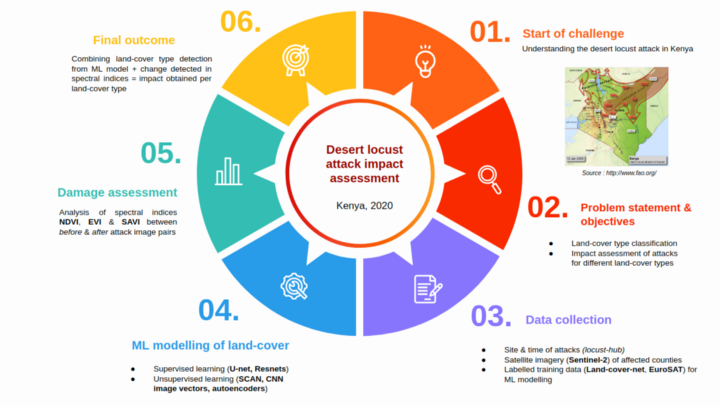
In this article, we will only highlight the main approaches we took for assessing the damage caused by the 2020 Kenya desert locust outbreak.
Data acquisition
We opted for Sentinel-2 images using the Google earth engine platform. Even though it doesn’t have the best spatial resolution (10m per pixel for most of the bands), Sentinel-2 has a decent temporal resolution compared to other open-source satellite imagery, with a revisit time of 5 days at the equator in cloud-free conditions. It also comes with multi-spectral bands that could provide valuable information and insights to analyze the vegetation loss, which is not captured by regular RGB channels. Thus, the Sentinel-2 source was our best option for this challenge.
Where to look
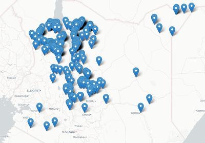
Before collecting the actual images, we first needed the coordinates for the regions that were attacked and the exact timing for those attacks. This information was available on the locust hub from FAO.
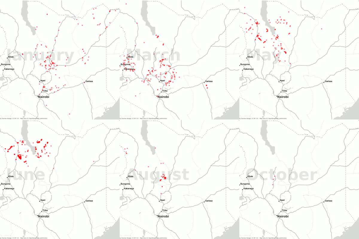
The goal was to have images before and after the attack to analyze and assess the damage the desert locust caused. We used the dates the locust hub provided to export images for each coordinate.
Here we faced another challenge — making a suitable selection of interval period for the attacks, i.e the temporal gap between before and after image at a location. This had to be done while also taking into account the temporal resolution for our source (five days in a clear weather condition), as well as the cloud conditions. We ended up choosing a range of a minimum of one day before/after an attack and up to 15 days. This gave us the best results when it came to image quality and quantity and also allowed us to ignore the seasonal effects.
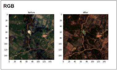
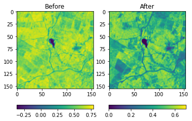
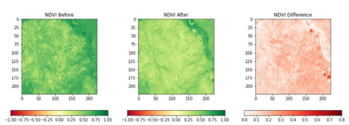
Given above, are the RGB and NIR-Red visualizations of a before-after image pair of an affected location in Kenya. In this example, we can spot the loss in vegetation with our naked eyes by comparison of the normalized difference vegetation index (NDVI) values.
To consider a pair of images, we needed them both to be usable. By that we mean the images have to consist of all the bands and with cloud coverage as little as possible. This resulted in discarding a good amount of images, but in the end, we were able to have 348 pairs of images to perform our analysis.
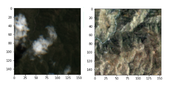
Another example from our collected data. This time we can see the clouds in the before image.
At this point, we had something to get us started with a basic understanding of the problem, and an idea about the effect of desert locust on some of the regions. But was that enough?
Getting more data for land cover classification
The data collected so far gave us insights on the loss of vegetation overall, but we needed more details. For example, to get the loss in vegetation per land cover type, we would first need to classify our land cover types and then perform the analysis on each one of these classes. And here comes the real power of AI and machine learning to help us drive these insights.
From Sentinel-2 we had our test data, but we still needed data to train our land cover classifier model. We had six main classes to take into account, as requested by the KRC — cropland, pastureland, bare soil, open water, forestland, and other-land. Considering the limited time of eight weeks in hand, and taking into account how time-consuming annotating such data could be, we needed a labeled dataset. This dataset had to have a similar resolution to the one we previously acquired for the damage assessment analysis and also similar characteristics when it comes to the topography and land types, and it had to be also free.
LandCoverNet Dataset
Not only was the data annotated, but it also has Africa as one of the main covered regions, and was collected from Sentinel-2. Again this was important because we would use this data to train our model and later test it on our before/after data, so they had to share the same properties to have consistent results, so this was perfect!
Here, it is worth mentioning that before LandCoverNet, we tried another labeled dataset which was Eurosat. The dataset was also taken from Sentinel-2, but the downfall was that it covered only regions within Europe, which proved to have quite different characteristics when testing the trained classifier on our collected images.
Supervised Learning
To build land cover classification ML models, we explored two approaches in the supervised learning category — image classification and semantic segmentation. Such classification models are first trained on a set of labeled images, to learn the class mappings with respect to image features and can then be used to predict the classes in test image inputs. In our case, the 6 classes of interest were provided by the KRC — cropland, pastureland, bare soil, open water, forestland, and otherland. The labeled data used in both the approaches were adapted to this set.
1. CNN image classification
Using transfer learning, we fine-tuned Resnet50 CNNs on the Eurosat dataset. Although it achieved a high accuracy of 98% on the Eurosat test data, the inference of this model performed poorly to our Sentinel-2 imagery of Kenya’s affected regions. One of the biggest plausible reasons for this behavior is the big gap between European land cover type and Kenyan vegetation. To bridge this difference, we had performed a label adaptation step between Eurosat land cover classes and expected classes in Kenya, which in turn, introduced fresh challenges. For example, all the images belonging to Industrial/Highway/Residential/Herbaceous Vegetation were mapped to one single class ‘Otherland’ (KRC label). This mapping process created a highly unbalanced dataset for training, and the resultant model predicted most of our images as ‘otherland’. Additionally, Eurosat did not have a ‘bare soil’ class, which is a common land cover in Kenya. As a result, Eurosat turned out impractical for our challenge.
2. Semantic Segmentation
To overcome the above challenges, we moved to land cover modeling using the LandcoverNet dataset which has classes similar to the African vegetation cover. This data has pixel-level labels. This required us to build a semantic segmentation model instead of the image classification. Segmentation is the process of classifying each pixel and assigning it to a particular label. Here we don’t separate instances of two same classes as we care only about each pixel category. It is mainly used to locate objects and boundaries in the images. Also, we can have an accurate view of an image as we can understand what is exactly in the image at pixel level view in a single class.
Moreover, semantic segmentation is quite useful in detecting and classifying the object in an image when we have more than one class in an image. This helped in our case as well, as our Sentinel-2 images had multiple classes within the same image.
3. U-Net Model
We used a pre-trained U-Net model for performing semantic segmentation. Originally introduced for biomedical image segmentation, U-net can perform fast and precise segmentation of images. Processing of 512×512 images takes less than a second on a GPU, which makes it very practical to use. We had used the Fast.AI framework, using the Google Colab platform. For training, we used 1980 images from the collected LandCoverNet data and used only 3 spectral bands (R, G, B). The original labels were also adapted to fit the KRC classes as shown below.
- Unknown, Artificial ground, Snow/ice = Otherland
- Cultivated Vegetation = Cropland
- (Semi) Natural Vegetation = Pasture land
- Natural Ground = Bare soil
- Water = Open water
- Woody Vegetation = Forestland
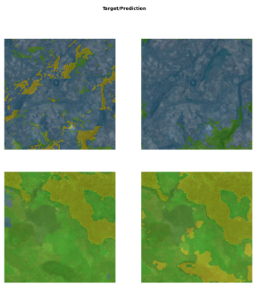
Due to the similarity between the labels, no significant imbalance was introduced. The U-net model achieved an impressive 81% accuracy in classifying the LandCoverNet data. Below, we can observe two targets/prediction pairs:
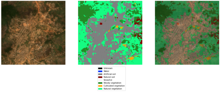
Having confidence in this modeling, we now applied it to classify our Sentinel-2 imagery. A sample predicted segmentation is shown below.
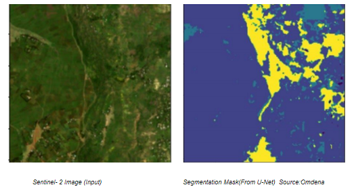
The segmentation masks and their prediction confidence were sufficiently high for us to next use them for the damage assessment section. However, before discussing them, we list here some ideas with which the segmentation modeling could be further improved in the future:
- Increasing the number of input images
- Fine-tuning model parameters
- Adding more spectral bands
- Increasing the number of training epochs
Unsupervised Learning
Before moving to the damage assessment section, we wanted to briefly touch upon the experiments we carried out during the initial phases of the project when labeled datasets for African vegetation were not yet available. During this time, we applied k-means clustering with various feature extraction techniques to the Sentinel-2 imagery of the affected regions. The images or pixels, which end up in the same cluster, would be more alike than those in other clusters. The different clusters could be considered to be representative of the different land-cover types and then be used for damage assessment.
We started with the simple Principal Component Analysis (PCA) for feature extraction. In this example shown, k-means was applied to the top three bands found to be the principal components in a sentinel-2 image having six bands.
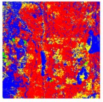
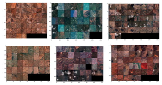
However, a limitation of such segmentation was that the clusters formed in one image would be different from the clusters found in other images. This would not be very reliable as we would like to identify the same classes across images. A possible strategy to overcome this was to perform PCA (followed by k-means) on a single large image covering the whole of Kenya. But, this turned out to be computationally very expensive and this approach was not pursued. Therefore, next, we moved to attempt image-level clustering. Three main techniques applied were — the SCAN algorithm, Image feature vectors from a pre-trained CNN, and auto-encoders. An example is shown below, using SCAN. Detailed results are omitted and can be read on our unsupervised article for this project.
How to use the clusters in our work
A major limitation with clustering is that although the images are grouped, they do not give any information about which cluster represents what type of land-cover. Therefore the next step was to annotate the clusters and map them to a land-cover class. In the initial stages, we attempted manual annotation, by visual observation of the cluster images. Later, we obtained the Land Use Land Cover (LULC) map of Kenya, 2019 (which differed from the land-cover types given KRC but was a good representation of Kenya land-cover type). As each Sentinel-2 image in any given cluster referred to geolocation, we plotted points of all the clusters on this map. Using majority voting of the land-cover type that most of the images in a cluster belonged to, clusters were assigned an overall class label. A sample plotting of images from the clusters of the VGG16 features are shown below:
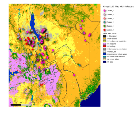
In the annotation step with the LULC map, we observed that more than one cluster was sometimes assigned the same label, therefore, indicating that clusters could be further merged. It implied that our database of the attack locations of Kenya does not contain six different land-cover types as expected by KRC. The clustering is thus expected to improve if carried out with an optimal value of k, using elbow methods, etc. Additionally, K-means being a hard clustering technique, any given image could belong to only a single cluster. As a result, the entire two km of land covered in an image in our project, would be categorized as a single land-cover type, whereas the ground reality could be that multiple land-cover types exist in that land covered in a single image. In future works, soft clustering methods (such as Fuzzy clustering) could be used. Therefore, in the later stages of the project when Land-Cover-Net labeled data was obtained, the U-net supervised modeling was pursued to perform semantic segmentation which overcame this limitation of image-level clustering.
Damage Assessment
Once the land cover types were classified the next step was to assess the impact of damage caused by desert locusts in these areas. Traditionally, damage assessment is made by collecting crop acreage, data from field surveys, farmers, etc., which is time-consuming and cost-intensive. We researched the current approaches that are used for impact assessment and how to incorporate them effectively in our existing ML pipeline.
How did we approach this?
Remote sensing for vegetation provides a cost-effective solution for vegetation condition monitoring by providing multi-temporal images. It is mainly done by obtaining the electromagnetic wave reflectance information from canopies using passive sensors. The reflectance of light from plants changes with its type, the water content in its tissues, and other intrinsic factors. Indices extracted from these spectra can be used for the vigor quantification of plants.
Vegetation indices
Vegetation interacts with solar radiation differently when compared to other natural materials. The vegetation spectrum reflects the green wavelength, strongly reflects the near-infrared wavelength (NIR), and absorbs red and blue wavelengths. The variation across the spectrum is further caused by carbon content, water content, nitrogen content, pigment, etc. The relationship to one another is known as vegetation indices.

Using vegetation indices we can get information about plant health, growth. It also helps to categorize different land covers as shown in the image above. Such Indices are based on three light spectra: UV region, Visible spectra & Near and Mid-infrared band. The three main vegetation indices which we considered are:
1. NDVI (Normalised Difference Vegetation Index)
A widely used index to measure vegetation condition or health. In other words, it is a simple indicator of photosynthetically active biomass.
How does NDVI work?
During photosynthesis plant, cells use carbon dioxide and sunlight to produce oxygen and sugar molecules. The primary pigment used in photosynthesis is chlorophyll and this absorbs visible light and reflects near-infrared light(NIR). By comparing NIR with visible light we can differentiate healthy plants from unhealthy ones. NDVI is used in this calculation, by measuring the difference between near-infrared light(NIR) and red light.
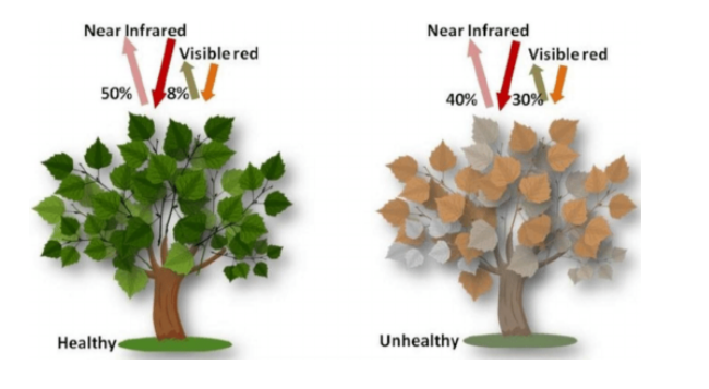
Very low values (<0.1) indicate barren rock or snow, water and high values (generally around 0.6 to 0.9) indicate dense vegetation, such as forests and crops. In the image below, we can see the evolution of NDVI values before and after the locust attacks. The after image clearly shows the degradation of vegetation, indicated by lower values of NDVI.
2. EVI (Enhanced Vegetation Index)
To address the soil and atmospheric limitations with NDVI, the Enhanced Vegetation Index (EVI) was introduced. Liu and Huete, after a detailed study, concluded that due to the interaction between soil and atmosphere increasing one may reduce the other. To simultaneously correct the soil and atmospheric effects, they built a parameter in this algorithm. EVI ranges from -1.0 to +1.0, with healthy vegetation generally between 0.20 to 0.80.
3. SAVI (Soil Adjusted Vegetation Index)
In areas where the soil is exposed and vegetation cover is low, NDVI values can be influenced by soil reflectance. SAVI was introduced to tackle this soil brightness factor. It is simply a modification of NDVI with an adjustment factor L for soil brightness. The default value for L is 0.5 and works well mostly. When L=0, NDVI=SAVI.
Calculating the degree of damage per land cover type
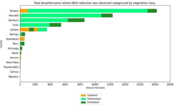
We obtained land-cover segmentation masks from the images taken before the locusts attack, using the U-net model. Then, we compared the vegetation indices of these segmented images with their temporal counterparts, i.e the after attack images. This analysis of index changes, allowed us to compute the total area damaged in hectares, the total area damaged per county, and vegetation cover damage per county. In the plots below, we report the NDVI changes observed. A similar trend of behavior was observed across EVI & SAVI indices as well, which validated our loss assessment.
NDVI analysis
The vegetation indices comparison illustrates that in terms of the amount of land (in hectares) affected, the most damaged land-cover type was pastureland, followed by forestland and then cropland. Laikipia county suffered the biggest loss in cropland, while the most loss in pastureland was seen in Turkana county. The counties that faced major damages combining the effect across all 3 land cover types were —Turkana, Marsabit, Samburu, Isiolo & Laikipia. However, in terms of the degree of damage suffered, most counties faced low damage (NDVI difference below 0.2) except Kirinyaga and Laikipia, where some high damage was seen.
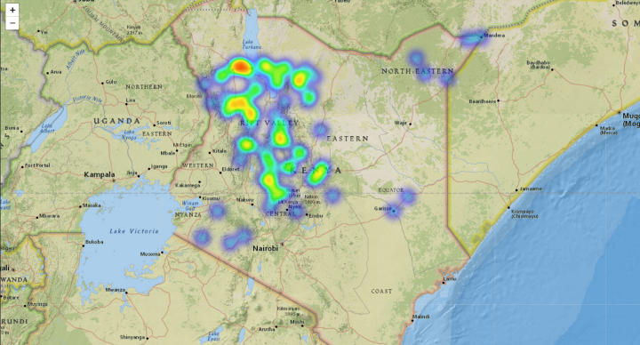
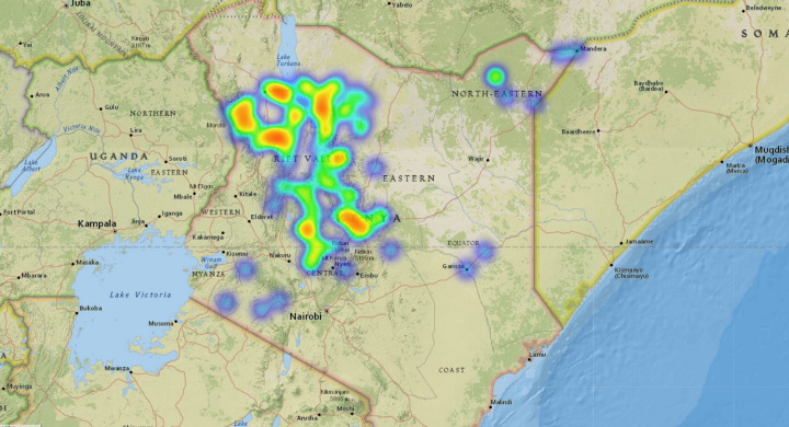
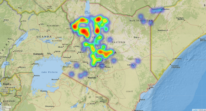
The following heatmaps highlight the geolocations of the damage. It is important to note in these plots that the resolution of the images is only 2km around each point, so there are possible gaps between the collected data points that were not part of this analysis. In the future, having bigger footprints could help improve this analysis.
Conclusion
The challenge was to leverage machine learning power and create a damage assessment tool for the desert locust attack. Data was one of the major obstacles, and even though we managed to overcome that, having a higher image resolution would have given far better insights as is the case with all machine learning problems. There is the “Copernicus Global Land Cover maps” dataset that we came across by the end of the challenge, and it could be used in the future, for training a classifier and comparing the different results.
There is also the possibility of trying other classification algorithms to enrich the outcome. And in fact, we did have some time to begin such an attempt by working on a U-net model that incorporates the NDVI band. After a few difficulties with the preparation of the dataset and the model to accept the fourth band, the model was finally working, but unfortunately time was not on our side and we couldn’t tune the model to have better results. Hence, we continued with our original U-net RGB model classifier. Another interesting approach was made by a collaborator was to predict the change in NDVI values for future attacks using the LSTM model. Working on different spectral indices could also provide more insights in this case.
This work was part of the Kenyan Red Cross efforts to offer relief for those affected by the large scale attacks. Being part of such a humanitarian mission, made us feel highly responsible and honored, motivating us to keep going to overcome the challenges along the way. We hope this work would provide first insights into the locust attack impact as was originally intended and pave the way for more future analysis in this direction.
